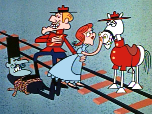
When writing a vision application, it’s easy to imagine noise within an image as a sinister character hiding in the shadows and fingering the end of a grease-slick mustache. "That’s a nice straight line you have there," his voice nasally dripping with malice. "It would be a shame if anything happened to it."
The problem is, he's right.
LabVIEW has a suite of powerful vision tools, most of which work fantastically well out-of-the-box. IMAQ Find Straight Edges 3 is unfortunately not one of them. It takes an image, a region of interest (ROI), some fitting parameters, and generates an array of rake points. Those rake points are used as the inputs to a linear fit, and if the fit is sufficiently good, it is presented as the output. There are a few fitting options, but none of them seem to handle noise very well.
The problem lies not with the rake points, but with how they are processed. A relatively small deviation in the rake points from a perfect line will systematically throw off the fit. The solution is to do the fitting ourselves.
To start, we use IMAQ Rake 3 to generate rake data using the same parameters as IMAQ Find Straight Edges 3. There are a few outputs, the most general of which is an array of search lines information. Each array element contains the endpoints of a given search line, as well as an array of found edge locations along the search line. We can then condition this data into an array of points (x,y) where x is the search line index and y is the distance between the start of the search line and a found edge.
Now we have an array of points on which to do linear regression. How do we learn from the mistakes of IMAQ Find Straight Edges 3? Stay tuned next time for the exciting conclusion in I Only Have Lines for You or An Array to Remember!
That was a Rocky and Bullwinkle joke.
I apologize.
Anyway, back to the answer: if we can measure the fitting error for a given point, we can weight it accordingly and devalue points with high error. The algorithm is as follows:
- Acquire conditioned rake data.
- Perform a linear regression with uniform weights.
- Until settled, or some max number of iterations has been reached:
- Generate weights as a function of error from the last fit.
- Refit with new weights.
The choice of a weight function should be something that decays quickly and monotonically to zero as abs(error) increases. Either a top hat or Gaussian centered at zero are good choices. Each family of functions is easily parameterized by a length scale, which makes for a great input parameter. Many other functions should work just fine, but these are simple to implement, and they perform well.
Once all of this is working, it’s easy to add further fitting options. A constraint on orientation can be achieved by constraining the slope of the linear regression. A line score for the output can be generated by measuring the average fitting error in various ways. It is useful to measure other fit properties: number of points with small error, line length, etc.
With all of this in place, we can start to get fancier with the analysis. A composite line score can be generated by taking a linear combination of functions of line metrics. We can run a window across an image, perform many fits, condense fits if appropriately close, and select the best results based on the composite score. We can do this for both rising and falling edges, correlating results to find rising/falling pairs based on similarity in orientation and separation. We can take these candidate pairs, and evaluate the pixel distribution of the region between them in order to verify that they bound a straight line.
Suddenly noise isn’t such a problem after all.
Learn more about DMC's LabVIEW programming services.