Have you ever wanted to create multiple PivotCharts in Excel showing different data from one table? I know I have, plenty of times!
This step-by-step tutorial will show you a quick and easy way to create PivotCharts that all refresh, update and filter together.
The first thing you'll want to do is open the applicable Excel sheet that you'd like to create PivotCharts in.
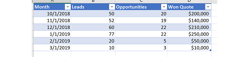
I created a sample table of data for this tutorial. From this table, I want three different charts showing me leads per month, opportunities per month and won quote amount per month.
First, I will create a new sheet in my same Excel workbook and navigate to any blank cell on this worksheet, which you can see in the image below.
Creating the PivotCharts
- Click on the top menu ribbon and navigate to insert.
- Click PivotChart.

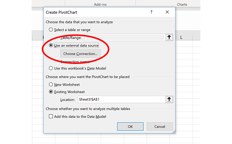
- The pop-up below will appear and you will choose the data you want to analyze for your Data Model.
- Click Use an external data source.
- Click Choose Connection.
- Click Tables.
- Choose the applicable table you'd like to create PivotCharts from. In my case, that is Table1.
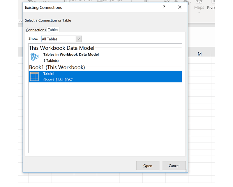
- Click Open.
- The same pop-up from before will appear again, and you will want to choose where you want the PivotChart to be placed.
- This should already be filled in for the cell you selected on your blank worksheet.
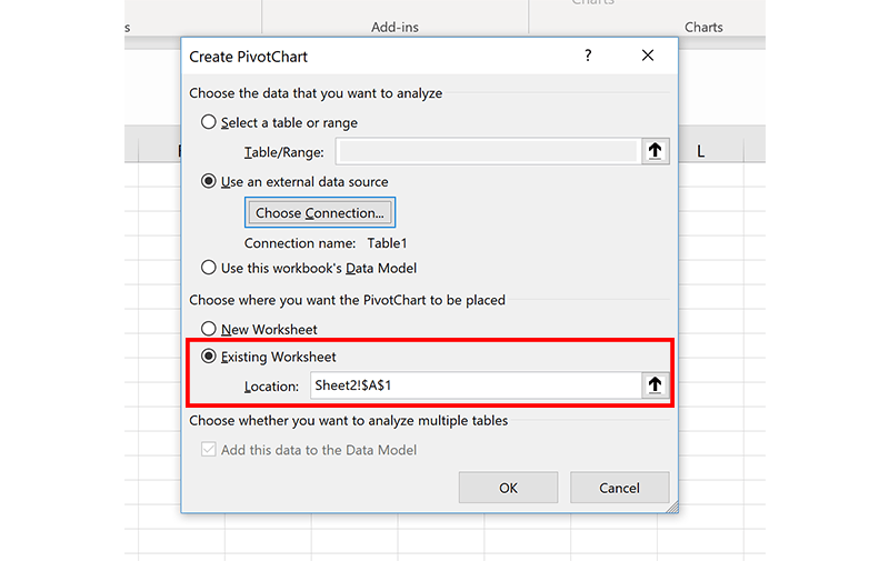
- Click Ok.
Now, the blank PivotChart field should appear.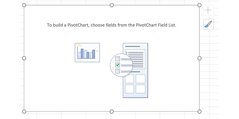
Putting data into the PivotChart
- On the right side of the worksheet, you should see the PivotChart Field List.
- You'll know that you have made the data connection successfully when there is "Table 1" at the top of the field list.
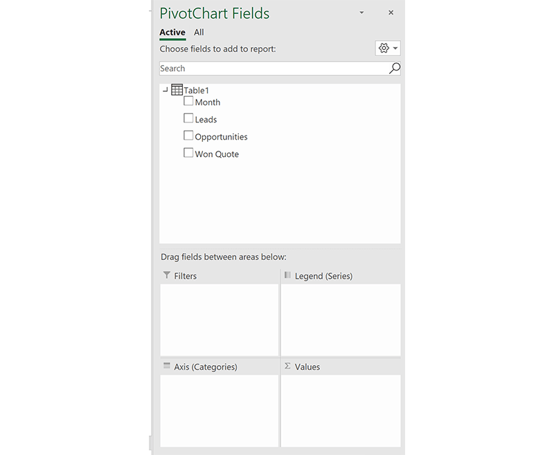
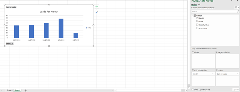
- In my case, I want the month to be my axis and leads to be my value.
- After inputting this into the field list, a PivotChart (shown below) will create in your worksheet.
Creating More Charts
I want to create the same type of graph, but with Opportunities as my value. All I have to do is copy and paste the leads graph into the same worksheet. Then, in the field list, change leads to opportunities in the value field and rename the graph.
I'll repeat this process for won quote amount.
Now, when you add more data into your original table, you will want to right-click on one of the PivotCharts and click refresh. All three charts will refresh with the new data.
Adding a Filter Slicer
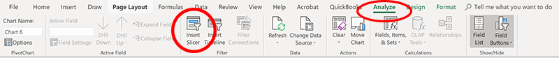
- Click on one of the charts and navigate to analyze in the top menu ribbon.
- Click insert slicer.
- Click whichever metric you'd like to filter by. In my case, I'd like to filter by month.
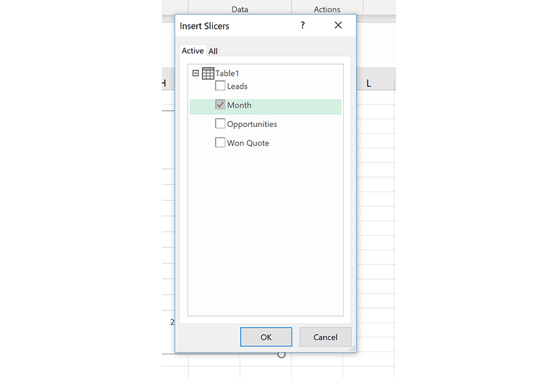
- Click Ok.
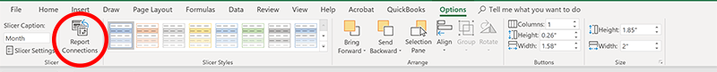
- To connect the filter slicer to all three PivotCharts, click your filter slicer and then click options in the top menu ribbon.
- Click Report Connections.
- Select all of the charts you'd like your filter to work on.
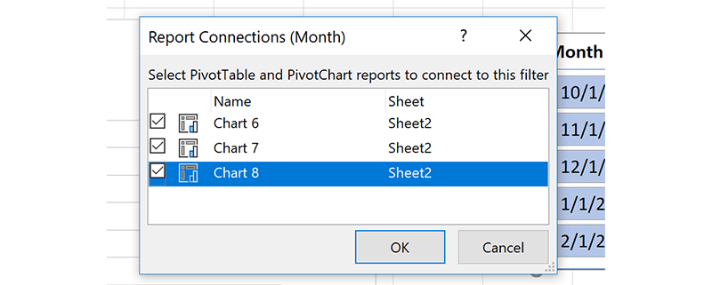
- Select Ok.
Now I can filter by month easily for all three graphs!
Check out this excel spreadsheet to see the end result of this tutorial.
PivotCharts are an awesome way to analyze your data even further. They can also help you set up multiple dashboards.
Learn more about DMC's Digital Workplace Solutions Services.